Neural Diffusion Equations

How it all started

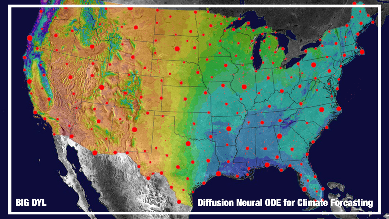
Climate modeling with neural diffusion equations started as a task for a capstone project at Yonsei University. After working on the neural partial differential equations (Neural PDE) project in BigDyl lab with Prof.Noseong Park, closely related to neural ODE and PINN, my interest was mainly focused on neural differential equations and physics-informed neural networks. During research for the project Neural PDE, I learned about climate modeling through the partial differential equation. However, attempts to directly apply Neural PDE to climate datasets or other spatiotemporal datasets were not successful as expected. This experience induced me to dig deeper into the recent successes of spatiotemporal models, which produced successful prediction results in climate forecasting/traffic forecasting tasks during the time.

So what is Neural Diffusion Equation?

Before diving into extensions and interpretations of the proposed NDE, I would like to briefly explain the concept (For those who want a more detailed explanation of the method, please refer to the paper, [PDF].).

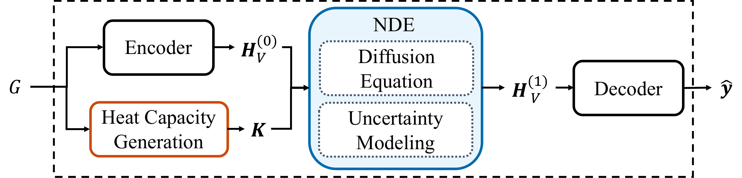
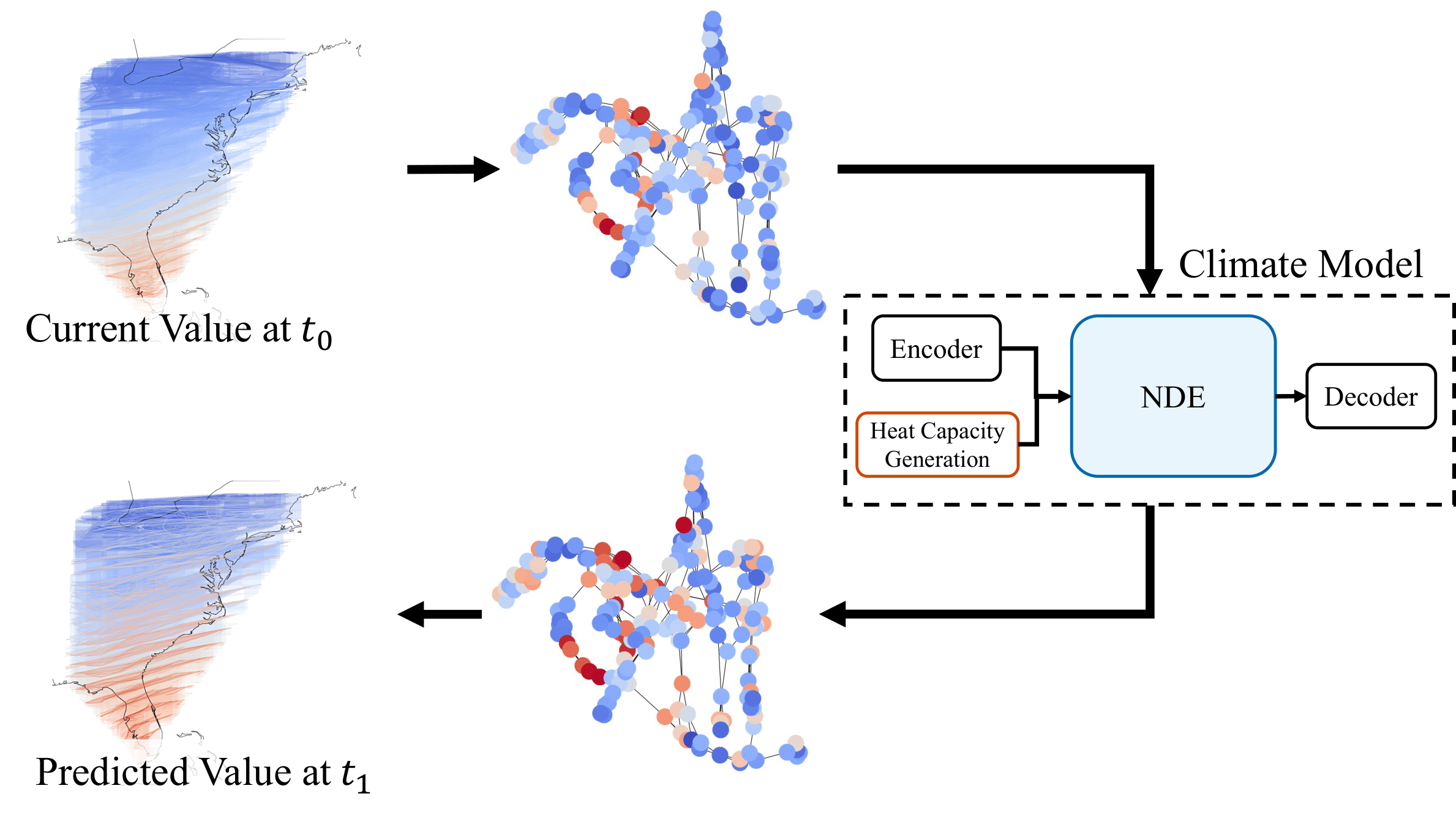
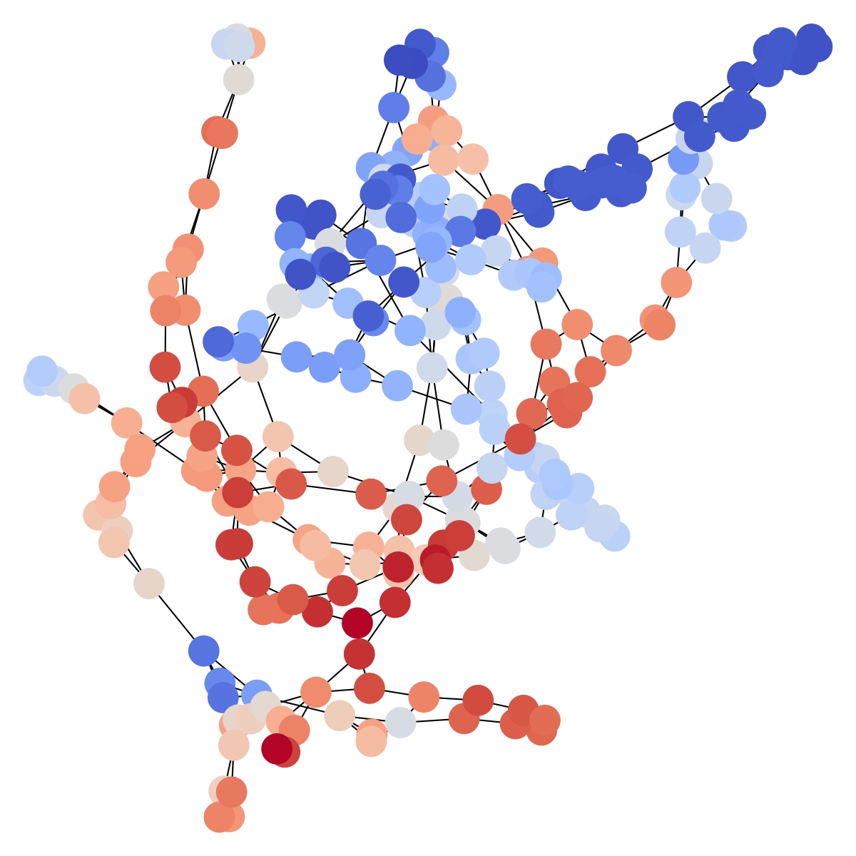
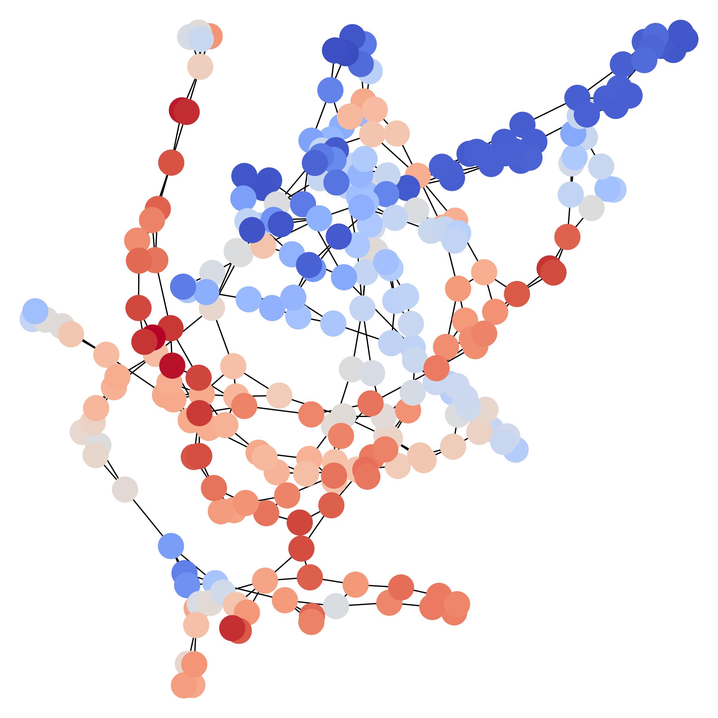
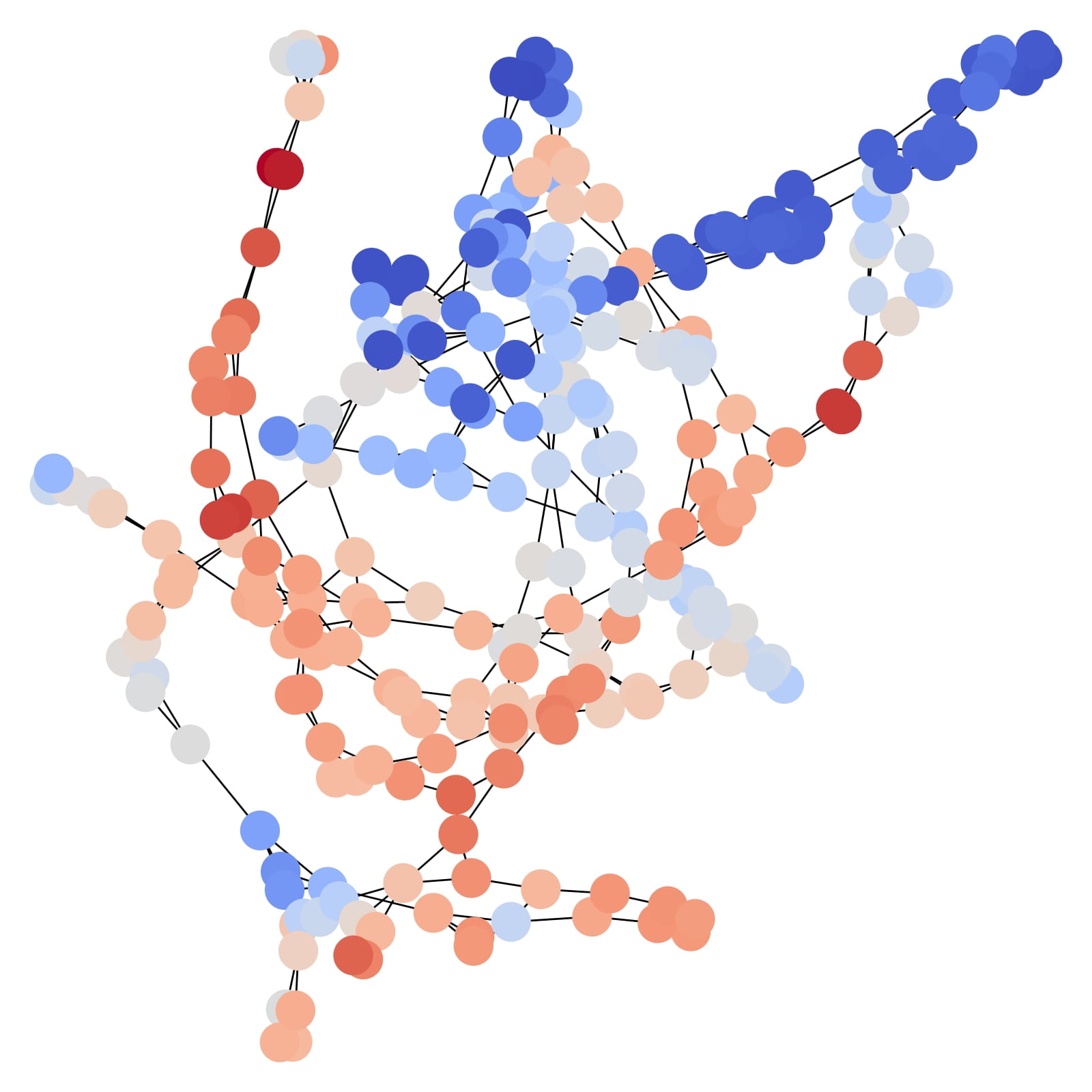
The weather stations (and their sensing values) are represented as a graph and our NDE predicts their future values. Given a graph \(G = (V, E) \) annotated with node and edge features, the core NDE layer evolves \(H_V^{(0)}\) to \(H_V^{(1)}\), followed by a decoding layer that produces predictions. Thus, the NDE layer consists of two parts: i) the diffusion equation and ii) the neural network-based uncertainty model \(f\).

Our model's diffusion equation consists of the predefined graph Laplacian matrix and learnable heat capacity matrix. There are four types for heat capacity modeling as follows.
1)Edge class: We learn a heat capacity coefficient for each class of edges when edge features are one-hot vectors. Edge classes are predefined by the land usage of each node(land).
2)Heat matrix: We learn a heat capacity matrix \(K ∈ R^{|V|×|V|}\).
3)Single coefficient: We learn a single heat capacity coefficient \(k ∈ R\).
4)Fixed coefficient: We consider the case of \(k=1\).
Uncertainty model \(f\) consists of a neural network with a few parameters for modeling noise in the given climate dataset to deal with the part that cannot be addressed by diffusion processes alone.

Perspectives of interpreting NDE

There are two ways to view the proposed concept NDE.

(1) Modeling diffusion equation with Neural ODE
(2) Continuous version of graph neural networks.

Graph Neural Networks (GNNs) operate by exchanging information between adjacent nodes in the form of message passing. This process is conceptually equivalent to the diffusion process, where nodes conduct diffusion through the edges. This analogy can be applied in various GNN based papers. Take, for example, simple graph convolution (SGC) [2]. SGC has the following layer definition. $$H(m) = S^mH(0) \tag3$$ where \(H\) is the node hidden matrix, and \(S^m\) is the \(m\)-th power of the symmetrically normalized adjacency matrix S with added self loops. Then, Eq.(2) can be derived from Eq.(3), as proven in our paper, where Eq.(2) becomes equivalent to Eq.(3) when the Euler method with a unit step size is used. This analogy of diffusion-based GNNs to continuous graph neural networks enables simple Euler solvers to be expanded to various solvers, such as the Dormand-Prince method or implicit solvers. Moreover, a neural network for uncertainty modeling can be applied side by side with a diffusion equation completing the equation for our NDE.

Where NDE leads us

Our method, therefore, can be viewed as where the study of physics informed neural networks and graph neural networks, and neural differential equations meet. This analogy also suggests that there are multiple ways to expand or change and reinvent the concept. Currently, my colleagues and I are working on not only its applications but also developing its theory.

Since numerous equations can be applied in this framework, a simple extension would be changing the differential equation. Advection-diffusion (or convection-diffusion) equation would be the most straightforward extension of our work, which also considers the direction of the graph. Since the graph structure and edge classes are maintained throughout our proposed training process, dynamic graphs or graph-structure learning can also be an advancement. Finally, controlled differential equations, a more general equation than an ordinary differential equation that uses the Riemman integral, can also be a great direction to advance. (Check on our new project STG-NCDE)

Currently, this project is under journal extension process.✨

References

[1]S. Seo and Y. Liu, “Differentiable physics-informed graph networks,” arXiv preprint, 2019[2]F. Wu, A. Souza, T. Zhang, C. Fifty, T. Yu, and K. Weinberger, “Simplifying graph convolutional networks,” in ICML. PMLR, 2019.